(1) Introduction to Causal Inference
Causal Data Science for Business Analytics
Hamburg University of Technology
Monday, 24. June 2024
Course Overview
Learning Goals
- Understand the difference between “correlation” and “causation”
- Understand the shortcomings of current correlation-based approaches
- Develop causal knowledge relevant for specific data-driven decisions
- Formalize intuition about causal relationships using a “language” of causality
- Derive causal hypotheses that can be tested with data
- Discuss the conceptual ideas behind state-of-the-art causal data science tools and algorithms
- Carry out causal data analyses with state-of-the-art tools
Map of Causality
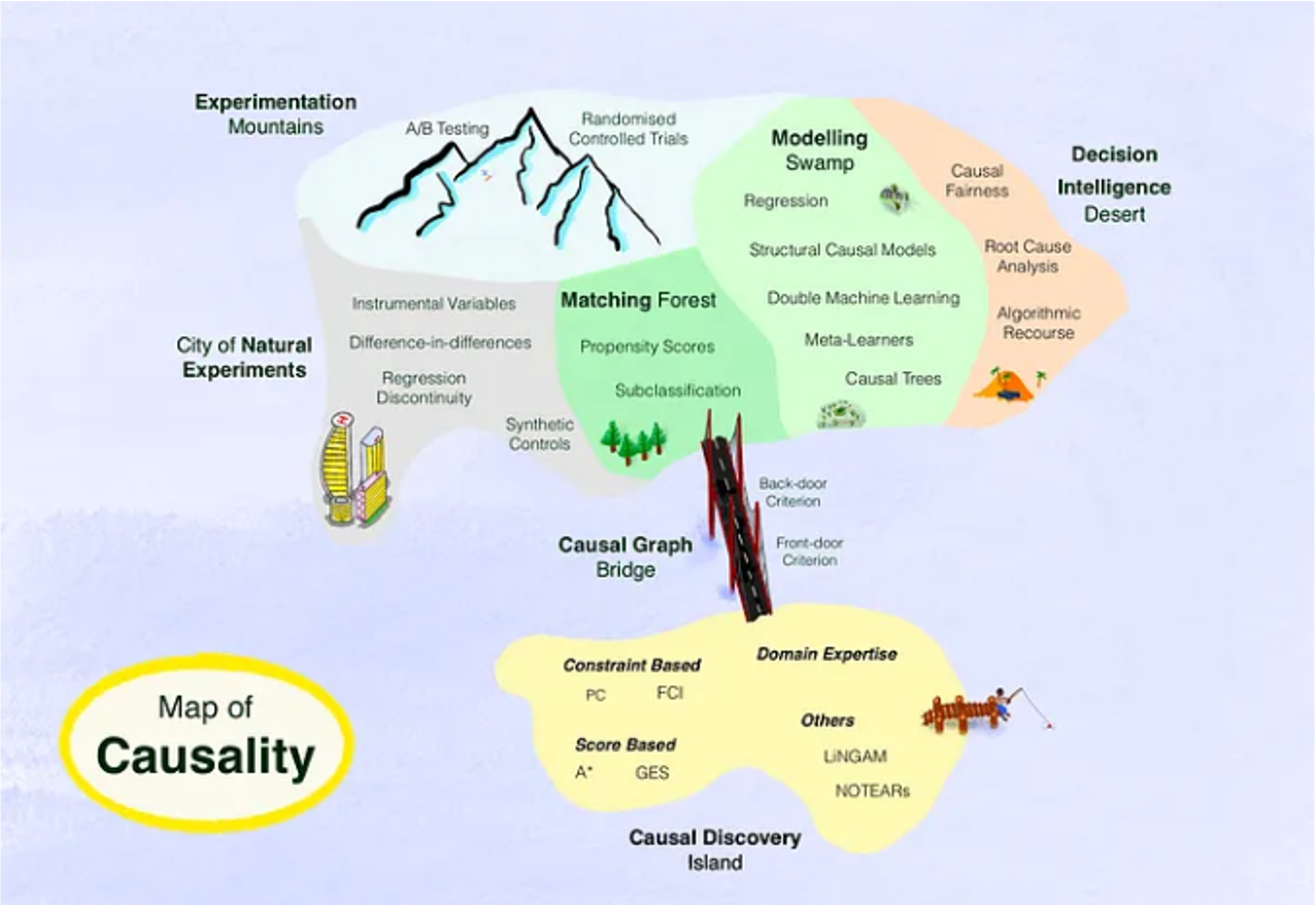
Source: https://towardsdatascience.com (2023).
Preliminary Schedule
| Session | Date | Topic |
|---|---|---|
| 1 | April 15 & 16 | Introduction to Causal Inference |
| 2 | April 22 & 21 | Graphical Causal Models |
| 3 | April 29 & 30 | Randomized Experiments |
| 4 | May 6 & 7 | Observed Confounding |
| 5 | May 13 & 14 | Double Machine Learning |
| - | May 20 & 21 | Holiday |
| 6 | May 27 & 28 | Effect Heterogeneity |
| 7 | June 3 & 4 | Unobserved Confounding & Instrumental Variables |
| 8 | June 10 & 11 | Difference-in-Difference |
| 9 | June 17 & 18 | Synthetic Control |
| 10 | June 24 & 25 | Regression Discontinuity |
| 11 | July 1 & 2 | Causal Mediation |
| 12 | July 8 & 9 | Further Topics in Causal Machine Learning |
Course Structure
Lecture - Causal Data Science:Monday, 11.30 - 13.00, Building D, Room D - 1.023Lab - Business Analytics with Causal Data Science:Tuesday, 15.00 - 16.30, Building O, Room O - 0.007
Examination:10 challenges related to each topic documented in a lab journal
Contact:Oliver Mork (oliver.mork@tuhh.de)
Course Literature
- Ding, Peng (2023). A First Course in Causal Inference. arXiv preprint arXiv:2305.18793.
- Facure, Matheus (2023). Causal Inference in Python - Applying Causal Inference in the Tech Industry. O’Reilly Media.
- Huber, Martin (2023). Causal analysis: Impact evaluation and Causal Machine Learning with applications in R. MIT Press, 2023.
- Neal, Brady (2020). Introduction to causal inference from a Machine Learning Perspective. Course Lecture Notes (draft).
- Angrist, J. D., & Pischke, J. S. (2014). Mastering metrics: The path from cause to effect. Princeton university press.
- Cunningham, Scott (2021). Causal Inference: The Mixtape, New Haven: Yale University Press.
- Gertler, Paul J., et al. (2016). Impact evaluation in practice. World Bank Publications.
- Hernán Miguel A., and Robins James M. (2020). Causal Inference: What If. Boca Raton: Chapman & Hall/CRC.
- Huntington-Klein, Nick (2021). The effect: An introduction to research design and causality. Chapman and Hall/CRC.
- Imbens, G. W., & Rubin, D. B. (2015). Causal inference in statistics, social, and biomedical sciences. Cambridge University Press.
- Mullainathan, Sendhil, and Jann Spiess. (2017). Machine Learning: An Applied Econometric Approach. Journal of Economic Perspectives, 31(2): 87–106.
- Pearl, Judea, and Dana Mackenzie (2018). The Book of Why. Basic Books, New York, NY.
- Pearl, Judea, Madelyn Glymour, and Nicholas P. Jewell (2016). Causal Inference in Statistics: A Primer. John Wiley & Sons, Inc., New York, NY.
- Peters, Jonas, Dominik Janzing, and Bernhard Schölkopf (2017). Elements of causal inference: foundations and learning algorithms. The MIT Press.
Course Motivation
Causality vs. Correlation
- Causality is central to human knowledge.
- Two famous quotes from ancient Greeks:
- “I would rather discover one causal law than be King of Persia.”
(Democritus) - “We do not have knowledge of a thing until we grasped its cause.”
(Aristotle)
- “I would rather discover one causal law than be King of Persia.”
- However:
- Classic statistics is about association rather than causation.
- Machine learning is about prediction rather than causation.
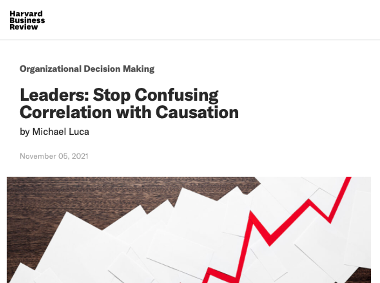
Causality vs. Correlation
- “Correlation does not imply causation.”
- “You can not prove causality with statistics.”
- But statistics is crucial for understanding causality:
- Formal language for causal inference.
- Methods to estimate causal effects.

Causality vs. Correlation
Causality vs. Correlation

Causality vs. Correlation
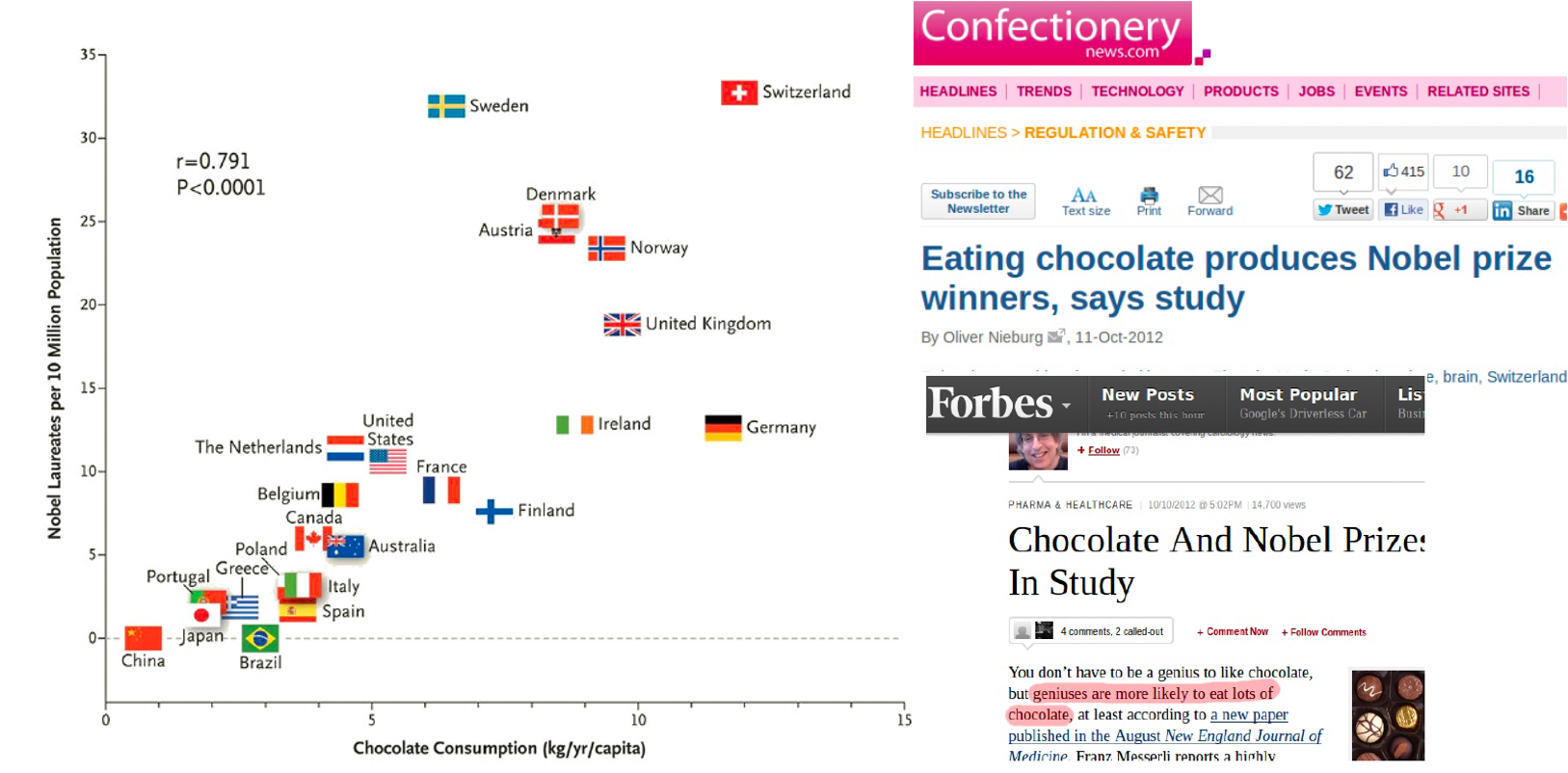
Source: Peters, Jonas. 2015. Causality: Lecture Notes, ETH Zurich.
Causality vs. Correlation
- Correlation, or better association, is not (entirely) causation, if there is confounding association due to a common cause, i.e. a confounder.
- E.g. drinking the night before is a common cause of sleeping with shoes on and of waking up with a headache:
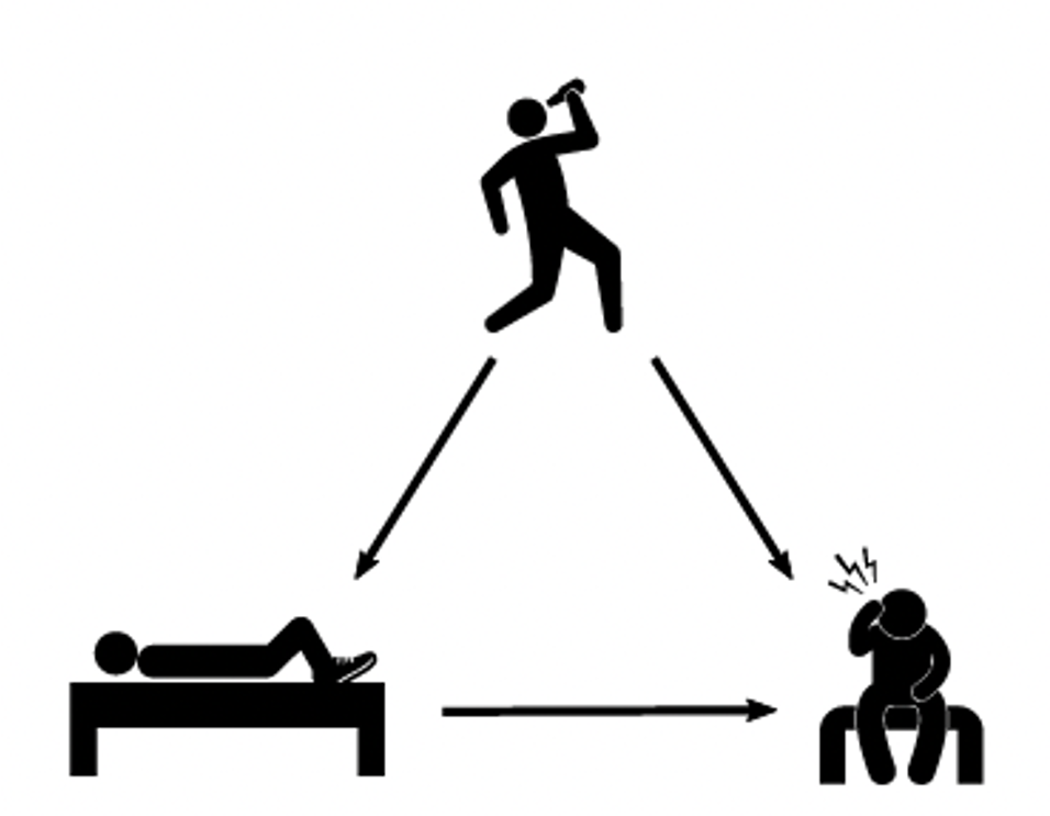
Source: Neal, Brady (2020). Introduction to causal inference from a Machine Learning Perspective. Course Lecture Notes (draft).
Causality vs. Correlation
- Correlation, or better association, is not (entirely) causation, if there is confounding association due to a common cause, i.e. a confounder.
- E.g. Consumers’ purchase intent is a common cause of the amount spent on search engine marketing (SEM) (esp. for branded vs. non-branded ads) and sales (especially for frequent consumers):
Show code
library(ggdag)
library(ggplot2)

coord_dag <- list(
  x = c(SEM = 0, Intent = 1, Sales = 2),
  y = c(SEM = 0, Intent = 1, Sales = 0)
)

dag <- ggdag::dagify(SEM ~ Intent,
                     Sales ~ SEM,
                     Sales ~ Intent,
                     coords = coord_dag)

dag %>%
  ggplot(aes(x = x, y = y, xend = xend, yend = yend)) +
  geom_dag_point(colour = "grey") +
  geom_dag_edges() +
  geom_dag_text(colour = "black", size = 5) +
  theme_dag(legend.position = "none")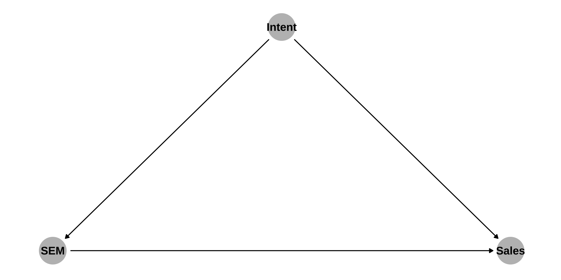
Simpson’s Paradox
Motivating Example: Gender Pay Gap (1)
“When Google conducted a study recently to determine whether
the company was underpaying women and minority groups, it found
that men were paid less money than women for doing similar work.”
- The study led Google to increase the pay of its male employees to fight this blatant discrimination of men.
- What’s going on here? Wasn’t Google just recently accused of discriminating against women, not men?
female employees.”
Motivating Example: Gender Pay Gap (2)
- Suppose we collected data on wages payed to 100 women and 100 men in company X.
- We observe the following average monthly salaries for women and men in management and non-management positions (case numbers in parentheses):
| Women | Men | ||
|---|---|---|---|
| Non-management: | $3,163.30 (87) | $3,015.18 (59) | |
| Management: | $5,592.44 (13) | $5,319.82 (41) |
- Our goal is to estimate the magnitude of the gender pay gap in company X. How should we tackle this problem?
Motivating Example: Gender Pay Gap (3)
- On average, women earn less in this example: \[ \left(\frac{87}{100} \cdot \$3163.30\right) + \left(\frac{13}{100} \cdot \$5592.44\right) - \left(\frac{59}{100} \cdot \$3015.18\right) + \left(\frac{41}{100} \cdot \$5319.82\right) \\ \approx -\$481 \]
- But in each subcategory women actually have higher salaries:
- Conditioning on job position gives the adjusted gender pay gap:
\[ \left(\frac{87 + 59}{200} \cdot \$148.12\right) + \left(\frac{13 + 41}{200} \cdot \$272.62\right) \approx \$181.74 \]
- Which estimate gives us a more accurate picture of the gender pay gap?
Motivating Example: Gender Pay Gap (4)
Show code
data <- data.frame(
  Salary = c(5319.82, 3015.18, 5592.44, 3163.30, 3960.08, 3479.09),
  Position = c("Management", "Non-Management", "Management", "Non-Management", "All Positions", "All Positions"),
  Gender = c("Male", "Male", "Female", "Female", "Male", "Female")
)

library(ggplot2)

data |>
  ggplot(aes(x=Gender, y=Salary, group=Position, colour=Position)) +
  geom_line() + geom_point() +
  theme_bw()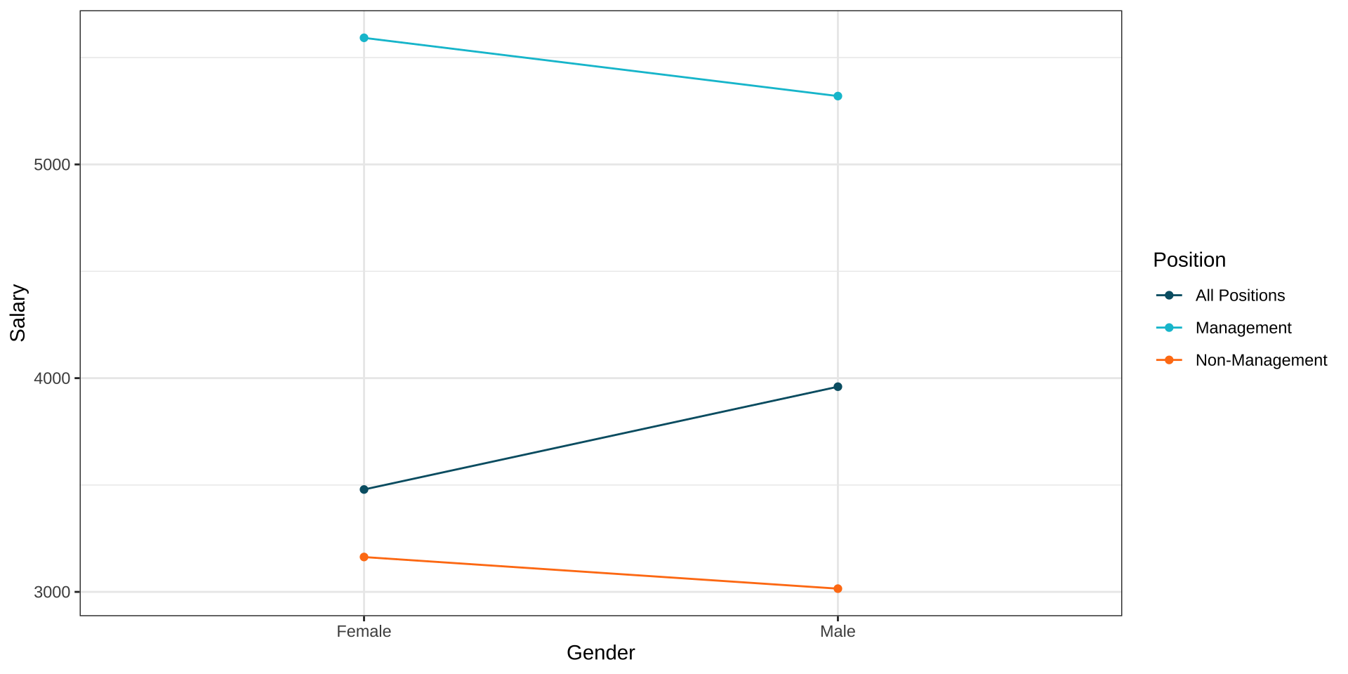
Simpson’s Paradox (1)
- The phenomenon that a statistical association, which holds in a population, can be reversed in every subpopulation is named after the British statistician Edward Simpson.
- Simpson’s paradox well-known, for example, in epidemiology and labor economics.
- In the gender pay gap example, the unadjusted gender pay (- $481) gap gives the right answer.
- But what about this example?
| Healthy Lifestyle | Unhealthy Lifestyle | ||
|---|---|---|---|
| Non-management: | $3,163.30 (87) | $3,015.18 (59) | |
| Management: | $5,592.44 (13) | $5,319.82 (41) |
Simpson’s Paradox (2)
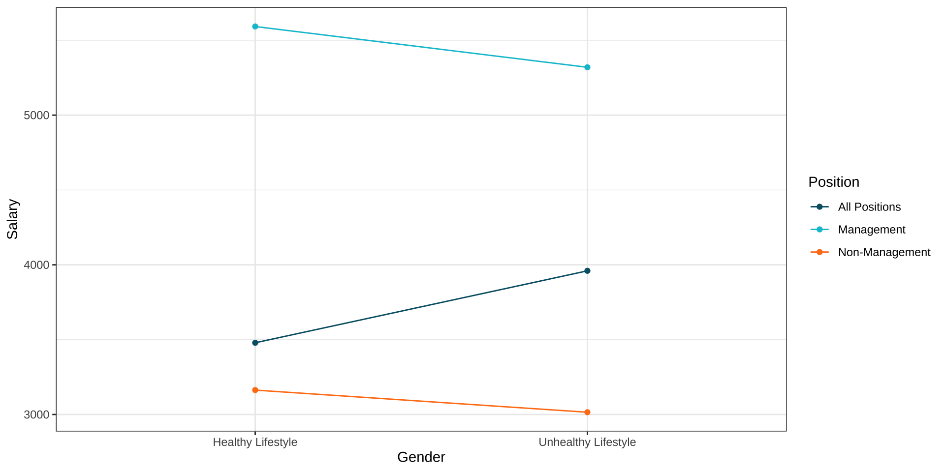
- Here, we would correctly infer that people with a healthy lifestyle earn more on average ($181.74).
Simpson’s Paradox (3)
- What is the difference between the two examples?
Show code
library(ggdag)

coord_dag <- list(
  x = c(Gender = 0, Management = 1, Salary = 2),
  y = c(Gender = 0, Management = 1, Salary = 0)
)

dag <- ggdag::dagify(Management ~ Gender,
                     Salary ~ Gender,
                     Salary ~ Management,
                     coords = coord_dag)

dag %>%
  ggplot(aes(x = x, y = y, xend = xend, yend = yend)) +
  geom_dag_point(colour = "grey") +
  geom_dag_edges() +
  geom_dag_text(colour = "black", size = 5) +
  theme_dag(legend.position = "none")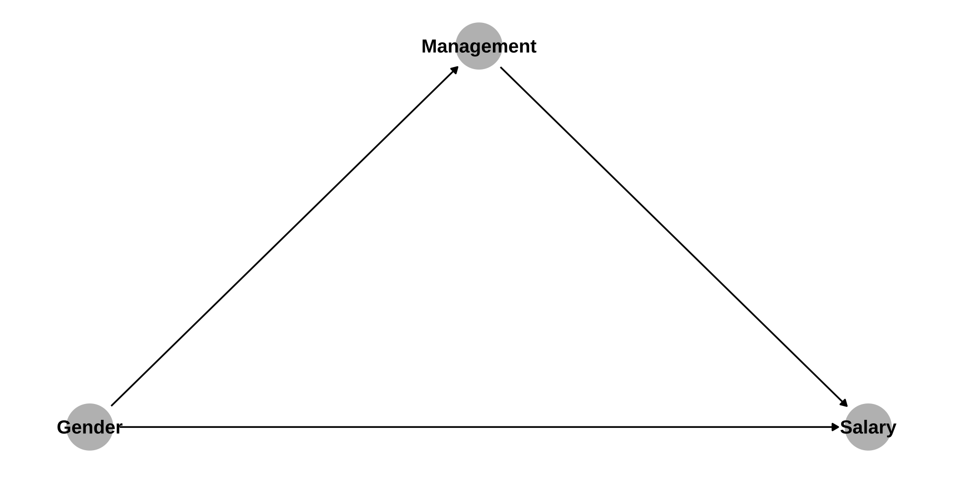
- Management as “mediator”
Show code
library(ggdag)

coord_dag <- list(
  x = c(Lifestyle = 0, Management = 1, Salary = 2),
  y = c(Lifestyle = 0, Management = 1, Salary = 0)
)

dag <- ggdag::dagify(Lifestyle ~ Management,
                     Salary ~ Lifestyle,
                     Salary ~ Management,
                     coords = coord_dag)

dag %>%
  ggplot(aes(x = x, y = y, xend = xend, yend = yend)) +
  geom_dag_point(colour = "grey") +
  geom_dag_edges() +
  geom_dag_text(colour = "black", size = 5) +
  theme_dag(legend.position = "none")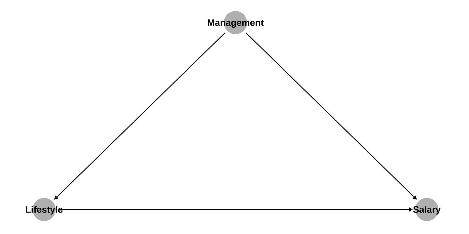
- Management as “confounder”
Simpson’s Paradox (4)
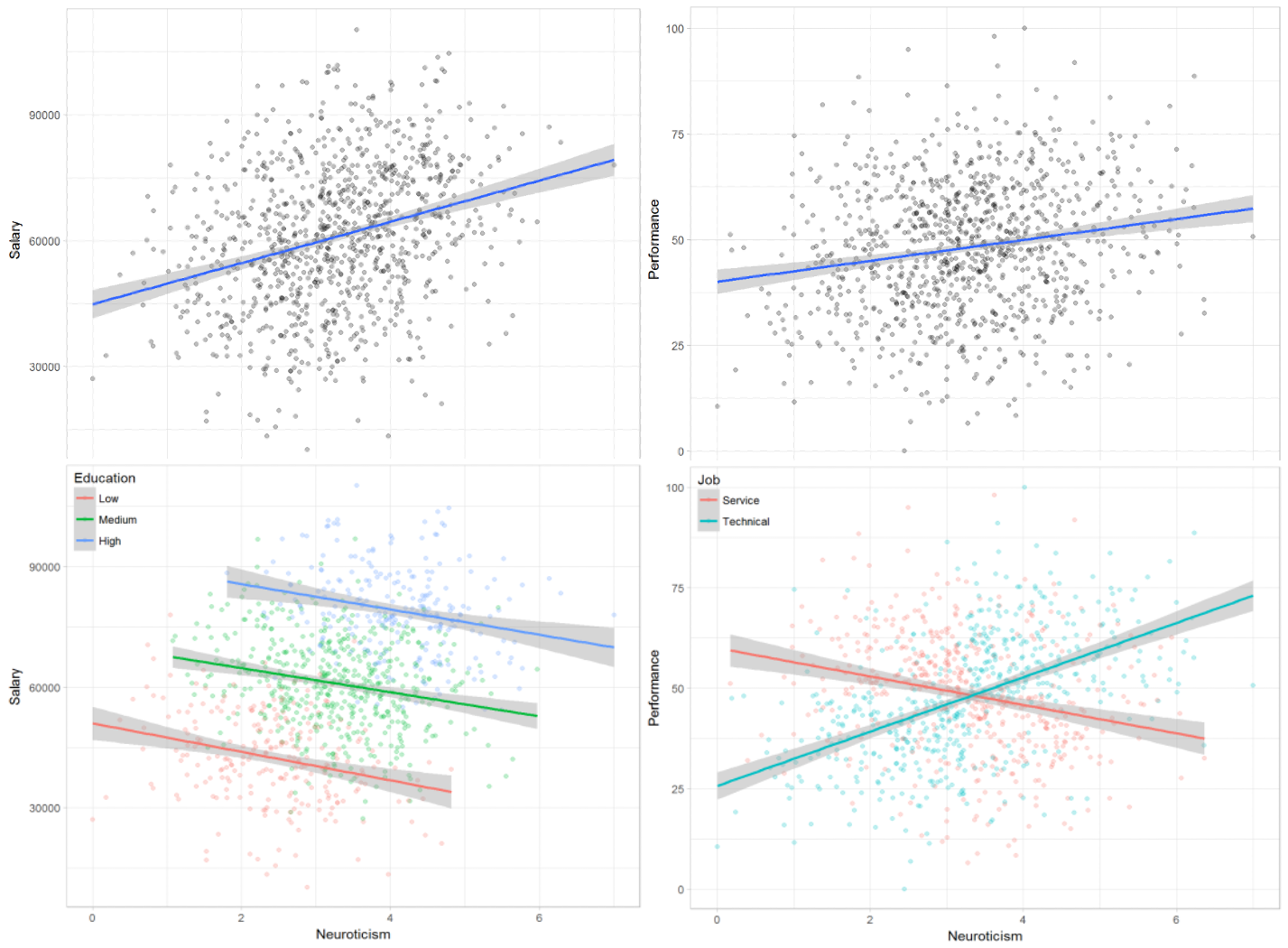
- Statistics alone doesn’t help us to answer this question.
- Note that the joint distribution of salaries is the same in both cases.
- Both problems are thus identical from a statistical point of view.
- Instead, we need to make causal assumptions in order to come to a conclusion here:
- Gender affects both a person’s salary level and job position.
- Whereas lifestyle affects salaries, but is itself affected by a person’s job position.
- After the course you will know how to incorporate this kind of causal knowledge in your analysis in order to solve all sorts of practical problems of causal inference.
Simpson’s Paradox (5)
Potential Outcomes
Experimentalists’ View of Causal Inference
- “No causation without manipulation.”
(Rubin, 1975; Holland, 1986) - (Thought) Experiments with manipulation; also called intervention or treatment.
- Treatments can be binary, continuous, or multi-valued.
- Examples:
- take a drug vs. don’t take a drug
- participate in a training program A vs B vs. don’t participate
- amount of money spent on advertising
- change race of job applicants? Resumes with African-American- or White-sounding names
(Bertrand and Mullainathan, 2004). - level of neuroticism?
- The potential outcomes framework
(Neyman, 1923; Rubin, 1974)is a way to formalize this idea.
Formal Notation of Potential Outcomes
- \(n\) experimental units indexed by \(i = 1, . . . , n\)
- \(Y\) is the outcome of interest.
- \(T_i\) is the (random) treatment variable for unit \(i\).
- Assume it can take two levels: \(t_i = 1\) for treatment and \(t_i = 0\) for control.
- \(Y_i(1)\) is the potential outcome for unit \(i\) if unit \(i\) receives treatment.
- \(Y_i(0)\) is the potential outcome for unit \(i\) if unit \(i\) does not receive treatment.
- The Individual Treatment Effect (ITE) for unit \(i\) is defined as:
- \(\tau_i = Y_i(1) - Y_i(0) \quad \forall \quad i = 1, . . . , n\).
Assumptions in the PO Framework (1)
For the potential outcomes and the ITE to be precisely defined, we need to make an initial set of assumptions:
Assumption 1: “No Interference”
Unit i’s potential outcomes do not depend on other units’ treatments.
\(Y_i(t_1,...,t_{i-1},t_i,t_{i+1},...t_n) = Y_i(t_i)\)
Assumption 2: “Consistency.”
There are no other versions of the treatment. Equivalently, we require that the treatment levels be well-defined, or have no ambiguity at least for the outcome of interest. If the treatment is \(T\), then the observed outcome \(Y\) is the potential outcome under treatment \(T\).
Formally, \(T = t => Y = Y(t)\) or equivalently \(Y = Y(T)\)
Assumption 3: “Stable Unit Treatment Value Assumption (SUTVA).”
Both Assumptions 1 and 2 hold: \(Y_i = Y(T_i)\)
Fundamental Problem of Causal Inference
- Typically, only one of those outcomes is actually observed for unit \(i\):
- \(Y_i = T_iY_i(1) + (1 − T_i)Y_i(0)\).
- The other one remains unobserved or counterfactual.
- This makes calculating the ITE \(\tau_i\) impossible.
| \(i\) | \(T_i\) | \(Y_i\) | \(Y_i(1)\) | \(Y_i(0)\) | \(Y_i(1) - Y_i(0)\) |
|---|---|---|---|---|---|
| 1 | 0 | 0 | ? | 0 | ? |
| 2 | 1 | 1 | 1 | ? | ? |
| 3 | 1 | 0 | 0 | ? | ? |
| 4 | 0 | 0 | ? | 0 | ? |
| 5 | 0 | 1 | ? | 1 | ? |
| 6 | 1 | 1 | 1 | ? | ? |
Getting Around the Fundamental Problem
- Does the Average Treatment Effect (ATE) help?
- Defined in terms of expectations:
- \(\tau = \mathbb{E}[\tau_i] = \mathbb{E}[Y_i(1) - Y_i(0)] = \mathbb{E}[Y_i(1)] - \mathbb{E}[Y_i(0)]\)
- Defined in terms of averages:
- \(\tau = \frac{1}{n} \sum_{i=1}^{n} [\tau_i] = \frac{1}{n} \sum_{i=1}^{n} [Y_i(1) - Y_i(0)] = \frac{1}{n} \sum_{i=1}^{n} [Y_i(1)] - \frac{1}{n} \sum_{i=1}^{n} [Y_i(0)]\)
- Still not computable, because we don’t know the counterfactuals.
Assumptions in the PO Framework (2)
- We need to make further assumptions to make progress.
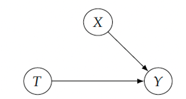
Assumption 4: “Ignorability / Exchangeability”.
Ignorability (of how people selected their treatment) is equivalent to random assignment into treatments.
Exchangeability means that observations in treatment and control group could be swapped, and one would still obtain the same outcomes. This implies that observations in groups are the same in all relevant aspects other than the treatment.
Formally, \((Y(1), Y(0)) \perp\!\!\!\perp T\).
ATE Identification - Intuition
- Using assumptions 4 and 2, we obtain the following simplification:
- \(\mathbb{E}[Y_i(1)] - \mathbb{E}[Y_i(0)] = \mathbb{E}[Y_i(1)|T_i=1] - \mathbb{E}[Y_i(0)|T_i=0] = \mathbb{E}[Y_i|T_i=1] - \mathbb{E}[Y_i|T_i=0]\)
- This implies the ATE to be obtainable as associational difference:
| \(i\) | \(T_i\) | \(Y_i\) | \(Y_i(1)\) | \(Y_i(0)\) |
|---|---|---|---|---|
| 1 | 0 | 0 | ? | 0 |
| 4 | 0 | 0 | ? | 0 |
| 5 | 0 | 1 | ? | 1 |
| 2 | 1 | 1 | 1 | ? |
| 3 | 1 | 0 | 0 | ? |
| 6 | 1 | 1 | 1 | ? |
- We can then estimate \(\mathbb{E}[Y_i|T_i=1] = 0.66\) and \(\mathbb{E}[Y_i|T_i=0] = 0.33\) and use these values to replace the missing counterfactuals.
- ATE is now identifiable in the sense that it can be computed from a purely statistical quantity.

Assumptions in the PO Framework (3)
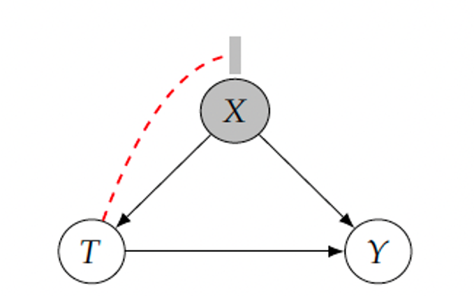
- Let’s make exchangeability more realistic, i.e. conditional on covariates, so that subgroups will be exchangable.
Assumption 5: “Conditional Exchangeability / Unconfoundedness”.
Formally, \((Y(1), Y(0)) \perp\!\!\!\perp T \, | \, X\).
Assumptions in the PO Framework (4)
- Conditioning on many covariates can also be detrimental, because we might end up conditioning on a zero probability event for some subgroups / values of X (division by zero)
Assumption 6: “Positivity / Overlap / Common Support”.
For all values of covariates \(x\) present in the population of interest (i.e. \(x\) such that \(P(X=x) > 0\)), we have \(0 < P(T=1|X=x) < 1\).
- There is a trade-off between positivity and unconfoundedness.
- Some models might be forced to extrapolate to regions without sufficient support by using their parametric assumptions.
Derivation of the Average Treatment Effect (ATE)
- With the assumptions of conditional unconfoundedness, positivity, consistency, and no interference, we can identify the ATE as:
Theorem 1: “Identification of the ATE”:
\(\tau = \mathbb{E}[Y_i(1)] - \mathbb{E}[Y_i(0)] = \mathbb{E_X}[\mathbb{E}[Y_i|T_i=1, X_i] - \mathbb{E}[Y_i|T_i=0, X_i]]\)
Derivation of the Average Treatment Effect (ATE)
- Proof:
\[\begin{align*} \tau = \mathbb{E}[\tau_i] &= \mathbb{E}[Y_i(1) - Y_i(0)] \\ &= \mathbb{E}[Y_i(1)] - \mathbb{E}[Y_i(0)] \\ & \text{(linearity of expectation)} \\ &= \mathbb{E}_X [\mathbb{E}[Y_i(1) \mid X_i]] - \mathbb{E}_X [\mathbb{E}[Y_i(0) \mid X_i]] \\ &\text{(law of iterated expectations)} \\ &= \mathbb{E}_X [\mathbb{E}[Y_i(1) \mid T_i = 1, X_i]] - \mathbb{E}_X [\mathbb{E}[Y_i(0) \mid T_i = 0, X_i]] \\ &\text{(unconfoundedness and positivity)} \\ &= \mathbb{E}_X [\mathbb{E}[Y_i \mid T_i = 1, X_i]] - \mathbb{E}_X [\mathbb{E}[Y_i \mid T_i = 0, X_i]] \\ &\text{(consistency)} \end{align*}\]
Other Causal Quantities
- The ATE is just one of many causal quantities that can be estimated using the PO framework.
“Average Treatment Effect on the Treated” (ATT):
\(ATT = \mathbb{E}[Y_i(1)|T_i=1] - \mathbb{E}[Y_i(0)|T_i=1]\)
“Conditional Average Treatment Effect” (CATE):
\(CATE = \mathbb{E}[Y_i(1)|X_i=x] - \mathbb{E}[Y_i(0)|X_i=x]\)
| Thank you for your attention! | |
 
|
|
Causal Data Science: (1) Introduction to Causal Inference