(2) Graphical Causal Models
Causal Data Science for Business Analytics
Hamburg University of Technology
Monday, 24. June 2024
Causal Graphs
Graphs
- Graph theory provides a useful mathematical language to think about causality.
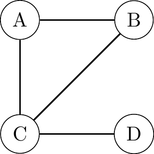
- A graph consists of vertices (or nodes) V and edges (or links) E. Vertices represent variables in the model and edges the connections between them.
- Edges can either be undirected or directed.
Directed Graphs
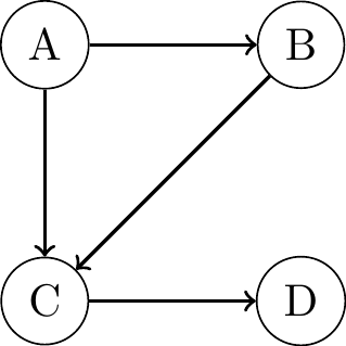
- Causal relationships are generally seen as asymmetric:
- If ‘A causes B’ is true, then ‘B causes A’ must be false.
- Therefore we’ll work with directed graphs most of the times.
- We’ll sometimes use terminology of kinship:
- A is parent of B.
- B is child of A.
- A is ancestor of D.
- D is descendant of A.
- A path is a sequence of edges connecting two vertices:
- \(B \gets A \to C \to D\) is a path from B to D.
- A path can go either along or against arrowheads.
- A path along the arrows is called directed: \(A \to C \to D\).
Directed Acyclic Graphs (DAGs)
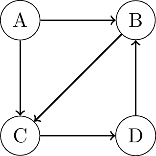
- A directed path from a node to itself is called
directed cycleorfeedback loop: \(B \to C \to D \to B\). - Graph with feedback loops is called cyclic, with no feedback loops acyclic.
- We focus on directed acyclic graphs (DAGs) in this course:
- exclude variables that influence themselves.
- Econometricians speak of recursive models that can be given a causal interpretation.

Bayesian Networks
- Probabilistic graphical models (not causal):
- Modelling the joint data distribution by factorizing with the chain rule of probability: \(P(x_1, x_2, \ldots, x_n) = P(x_1) \prod_{i} P(x_i \mid x_{i-1}, \ldots, x_1)\)
- n = 4: \(P(x_1, x_2, x_3, x_4) = P(x_1)P(x_2 \mid x_1)P(x_3 \mid x_2, x_1)P(x_4 \mid x_3, x_2, x_1)\)
- \(P(x_4 \mid x_3, x_2, x_1)\) alone requires \(2^3 - 1 = 8\) parameters = > Focus on local dependencies:
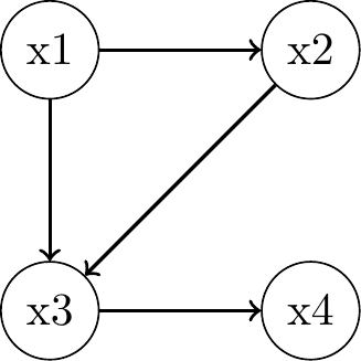
\(P_{joint} = P(x_1)P(x_2 \mid x_1)P(x_3 \mid x_2, x_1)P(x_4 \mid x_3)\)
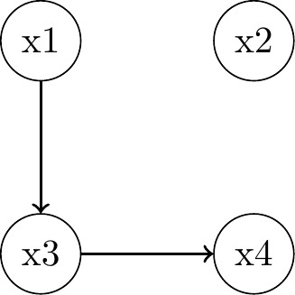
\(P_{joint} = P(x_1)P(x_2)P(x_3 \mid x_1)P(x_4 \mid x_3)\)
Bayesian Networks: Assumptions
Given a probability distribution and a corresponding DAG, we can formalize the specification of local (in-) dependencies with:
Assumption 2.1: “Local Markov Assumption”
Given its parents in the DAG, a node X is independent of all its non-descendants.
It follows:
Definition 2.1: “Bayesian Network Factorization”
Given a probability distribution \(P\) and a DAG \(G\), \(P\) factorizes according to \(G\) if:
\(P(x_1, x_2, \ldots, x_n) = \prod_{i} P(x_i \mid pa_i)\)
with \(pa_i\) denoting the parents of node \(i\) in \(G\).
Then \(P\) and \(G\) are called Markov compatible.
Assumption 2.2: “Minimality Assumption”
- Given its parents in the DAG, a node - is independent of all its non-descendants.
- Adjacent nodes in the DAG are dependent.
Causal Graph: Assumption
We need a further assumption to go from associations to causal relationships in a DAG:
Definition 2.2: “What is a cause?”
A variable X is said to be a cause of a variable Y if Y can change in response to changes in X.
An outcome variable Y listens to X.
Assumption 2.3: “(Strict) Causal Edge Assumption”
In a directed graph, every parent is a direct cause of all its children.
This assumption is “strict” in the sense that every edge is active, just like in DAGs that satisfy minimality.
Graph Building Blocks
Graph Building Blocks
- Understanding the flow of association and causation in DAGs based on minimal building blocks:
Two unconnected nodes:\(P(x_1, x_2) = P(x_1) P(x_2)\)

Two connected nodes:\(P(x_1, x_2) = P(x_1) P(x_2 \mid x_1)\)

Chain:

Fork:
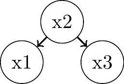
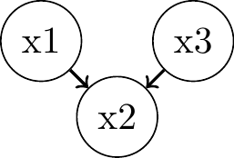
Immorality:
Chains


- \(x_1\) and \(x_3\) are
associatedthrough \(x_2\)- flow of association is symmetric whereas the flow of causality is directed
"Local Markov Assumption": we can block the associative path by conditioning on the parent \(x_2\)- \(x_1 \perp\!\!\!\perp x_3 | x_2\)
- => \(P(x_1, x_3 | x_2) = P(x_1 | x_2) P(x_3 | x_2)\)
- Proof?
Chains: Proof
"Bayesian network factorization"of chains:- \(P(x_1, x_2, x_3) = P(x_1) P(x_2 | x_1) P(x_3 | x_2)\)
"Bayes' rule":- \(P(x_1, x_3 | x_2) = \frac{P(x_1, x_2, x_3)}{P(x_2)}\)
- So that:
- \(P(x_1, x_3 | x_2) = \frac{P(x_1) P(x_2 | x_1) P(x_3 | x_2)}{P(x_2)}\)
"Bayes' rule"twice more:- \(P(x_2 | x_1) = \frac{P(x_1, x_2)}{P(x_1)}\) and \(P(x_1 | x_2) = \frac{P(x_1, x_2)}{P(x_2)}\)
- So that we finally obtain q.e.d.:
- \(P(x_1, x_3 | x_2) = \frac{P(x_1, x_2)}{P(x_2)} P(x_3 | x_2) = P(x_1 | x_2) P(x_3 | x_2)\)
Forks
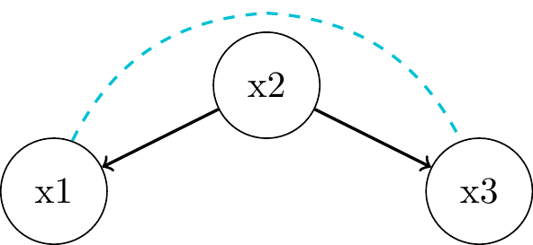
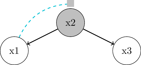
- \(x_1\) and \(x_3\) are
associatedthrough \(x_2\) as common cause orconfounder "Local Markov Assumption": we can block the associative path by conditioning on parent \(x_2\)- \(x_1 \perp\!\!\!\perp x_3 | x_2\)
- => \(P(x_1, x_3 | x_2) = P(x_1 | x_2) P(x_3 | x_2)\)
- Proof? Do try this sh.. at home!
Immoralities and Colliders
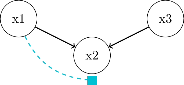
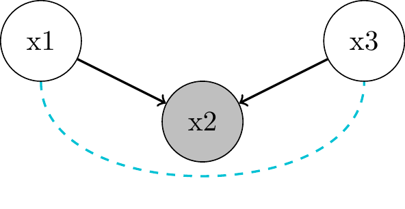
- no association in the first place: \(x_1 \perp\!\!\!\perp x_3\)
- no common cause (“confounder” like in a fork)
- neither is \(x_3\) a descendant of \(x_1\) (like in a chain)
- \(x_1\) and \(x_3\) are unrelated things contributing to \(x_2\)
- \(x_2\) acts as a
"collider"that blocks the path between \(x_1\) and \(x_3\)- but only if we do not condition on \(x_2\)
Immoralities and Colliders: Proof
"Bayesian network factorization"of immoralities:- \(P(x_1, x_2, x_3) = P(x_1)P(x_3)P(x_2 \mid x_1, x_3)\)
- Marginalizing out \(x_2\) (assuming discrete variables):
- \(P(x_1, x_3) = \sum_{x_2}P(x_1)P(x_3)P(x_2 \mid x_1, x_3) = P(x_1)P(x_3) \sum_{x_2}P(x_2 \mid x_1, x_3)\)
- Since summing over all possible values of the conditional probability \(P(x_2 \mid x_1, x_3)\) equals 1, we obtain q.e.d.:
- \(P(x_1, x_3) = P(x_1)P(x_3)\)
Immoralities and Colliders: Example
Looksandtalentare independent of each other in the general population- but both contribute to success (e.g. being casted as an actor, getting funding as founder, being in a relationship)
- in a selected sample of (un-) successful actors, looks and talent become negatively associated
- conditioning on success (by selecting a subsample) creates a
selection bias(orBerkson's paradox)
Immoralities and Colliders: Numerical Example
Data generating process (dgp): \(x_1 \sim N(0, 1), \quad x_3 \sim N(0,1), \quad x_2 = x_1 + x_3\)Covariance in the population:
\[\begin{align*} \text{Cov}(x_1, x_3) &= \mathbb{E}[(x_1 - \mathbb{E}[x_1])(x_3 - \mathbb{E}[x_3])] \\ &= \mathbb{E}[x_1x_3] \quad (\text{zero mean})\\ &= \mathbb{E}[x_1]\mathbb{E}[x_3] \quad (\text{independent}) \\ &= 0 \end{align*}\]
- Conditional covariance is the expected value of the product \(x_1x_3\), conditioned on \(x_2\) being equal to some value \(x\):
\[\begin{align*} \text{Cov}(x_1, x_3 | x_2 = x) &= \mathbb{E}[x_1x_3 | x_2 = x] \\ &= \mathbb{E}[x_1(x - x_1)] \quad (\text{substituting x_3 by x - x_1 as per dgp}) \\ &= x\mathbb{E}[x_1] - \mathbb{E}[x_1^2] \quad (\text{x is constant and expectations linear}) \\ &= -1 \quad (\text{E(x_1) = 0 and E(x_1*x_1) = Var(x_1) = 1}) \end{align*}\]
Immoralities and Colliders: Numerical Example
Show code
library(tidyverse)
library(ggplot2)
library(ggpubr)

# simulate data
set.seed(123) # for reproducibility
looks <- rnorm(1000)
talent <- rnorm(1000)
x <- talent + looks
group <- 1 * (x > quantile(x, c(.75)))

# create a dataframe
df <- data.frame(looks, talent, group) %>%
  mutate(group = if_else(group == 1, "With Job", "Without Job")) %>%
  add_row(looks = Inf, talent = -Inf, group = "Overall")

# plot
ggplot(df, aes(x = looks, y = talent)) +
  geom_point(aes(color = group)) +
  geom_smooth(method = "lm", se = FALSE, formula = y ~ x, aes(color = "Overall")) + # Regression line for all data
  geom_smooth(data = subset(df, group == "With Job"), method = "lm", se = FALSE, formula = y ~ x, aes(color = "With Job")) +
  geom_smooth(data = subset(df, group == "Without Job"), method = "lm", se = FALSE, formula = y ~ x, aes(color = "Without Job")) +
  stat_regline_equation(aes(label = ..eq.label.., color = as.factor(group)), formula = y ~ x) +
  stat_regline_equation(aes(label = ..eq.label.., color = "Overall"), formula = y ~ x) +
  labs(color = "Group") +
  theme(legend.position = "bottom")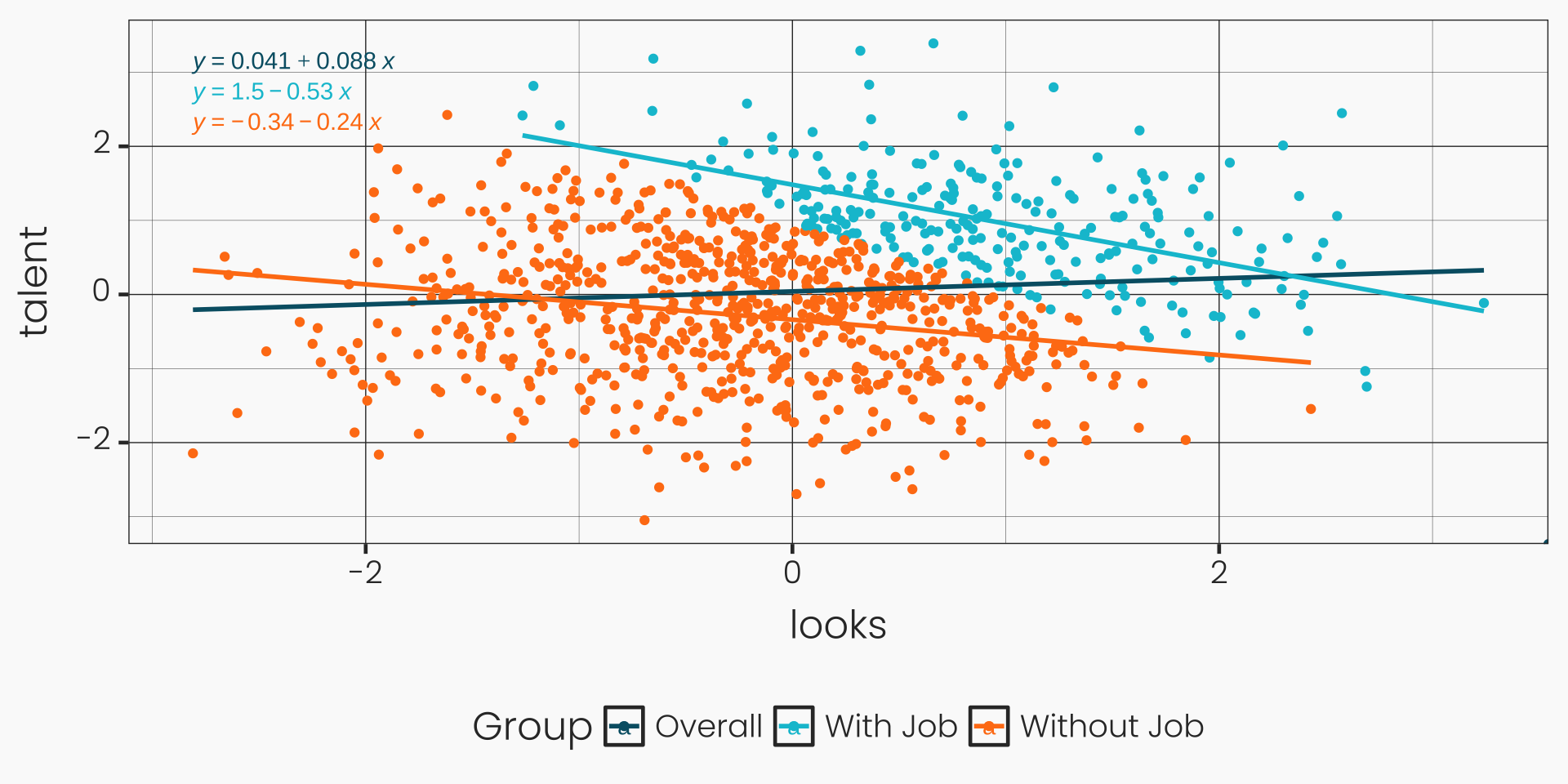
Descendants of Colliders
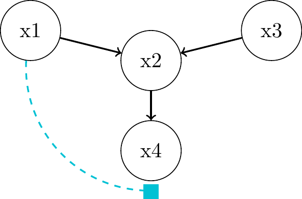
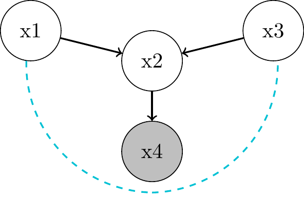
d-Separation
d-Separation
- So far we only looked at graphs containing three variables. Can we somehow generalize these criteria?
Definition 2.3: “Blocked Path”
A path \(p\) between nodes \(X\) and \(Y\) is blocked by a (potentially empty) conditioning set \(Z\) if either of the following is true:
\(p\) contains a chain of nodes \(... \rightarrow W \rightarrow ...\) or a fork \(... \leftarrow W \rightarrow ...\), and \(W\) is conditioned, i.e. \(W \in Z\).
\(p\) contains an immorality \(... \rightarrow W \leftarrow ...\), and the collider \(W\) is not conditioned, i.e. \(W \notin Z\).
Definition 2.4: “d-Separation”
Two nodes \(X\) and \(Y\) are d-separated by a set of nodes \(Z\) if all of the paths between \(X\) and \(Y\) are blocked by \(Z\).
d-Separation
- If two nodes are d-separated, and not d-connected, the variables they represent are independent.
Theorem 2: “Global Markov Assumption”
Given that \(P\) is Markov compatible with respect to \(G\) (satisfies the local Markov assumption), if \(X\) and \(Y\) are d-separated in \(G\) conditioned on \(Z\), then \(X\) and \(Y\) are independent in \(P\) conditioned on \(Z\).
Formally, \(X \perp\!\!\!\perp_{G} Y \,|\, Z \implies X \perp\!\!\!\perp_{P} Y \,|\, Z\).
d-Separation Practice 1
Show code
library(ggdag)
library(ggplot2)
dag <- dagify(
  # relationship for each node
  W ~ Z,
  W ~ X,
  Y ~ X,
  U ~ W,
 # Location of each node
  coords = list(
    x = c(Z = 0, W = 1, X = 2, Y = 3, U = 1),
    y = c(Z = 0, W = -0.5, X = 0, Y = 0, U = -1)
  )
)

dag %>%
  ggplot(aes(x = x, y = y,
             xend = xend, yend = yend)) +
  geom_dag_text(color = "black") +
  geom_dag_edges() +
  geom_dag_point(shape = 1) +
  theme_dag()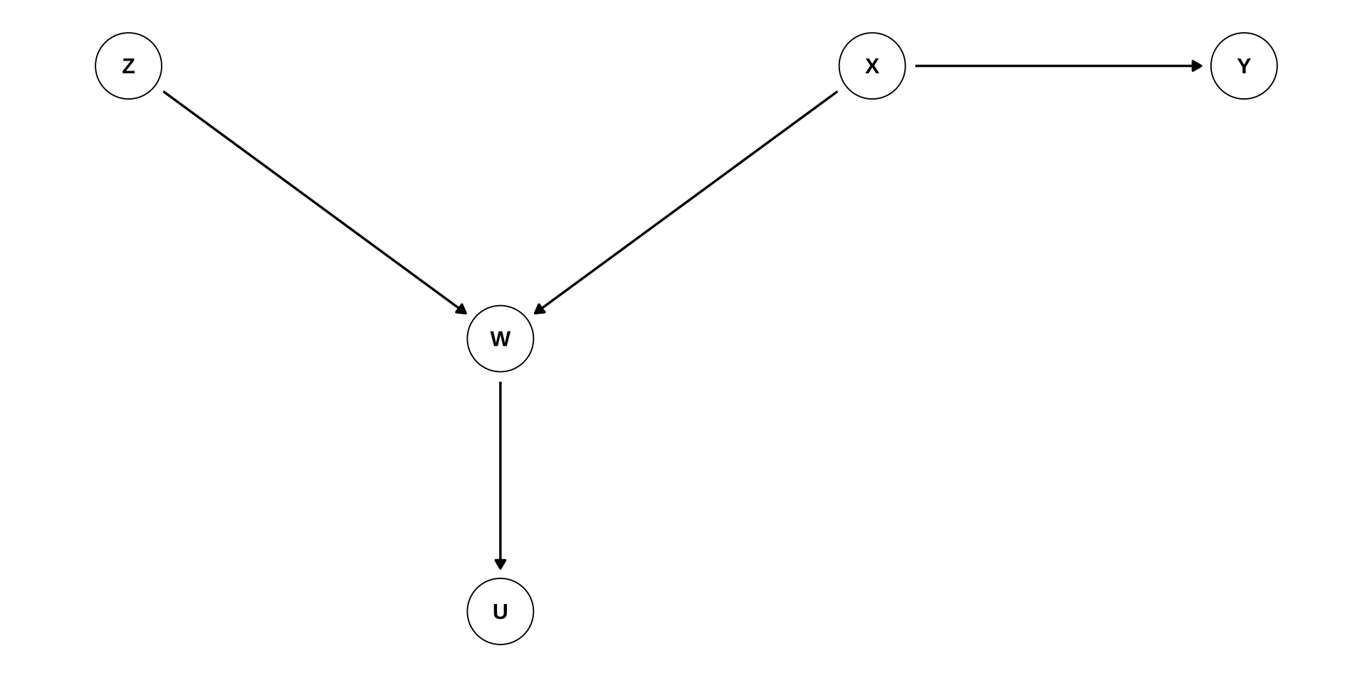
- \(Z\) and \(Y\)
d-separatedconditional on- \(\emptyset\) ? 2. \(\{W\}\) ? 3. \(\{U\}\) ? 4. \(\{W, X\}\) ?
d-Separation Practice 2
Show code
library(ggdag)
library(ggplot2)
dag <- dagify(
  Y ~ M2 + X3 + W3,
  W3 ~ W2,
  W1 ~ W2,
  T ~ W1,
  M1 ~ T,
  M2 ~ M1,
  X1 ~ T,
  X3 ~ Y,
  X2 ~ X1 + X3,
  coords = list(
    x = c(T = 0, W1 = 1, W2 = 1.5, W3 = 2, M1 = 1, M2 = 2, Y = 3, X1 = 1, X2 = 1.5, X3 = 2),
    y = c(T = -1, W1 = 0, W2 = 0.5, W3 = 0, M1 = -1, M2 = -1, Y = -1, X1 = -2, X2 = -2.5, X3 = -2)
  )
)


dag %>%
  ggplot(aes(x = x, y = y,
             xend = xend, yend = yend)) +
  geom_dag_text(color = "black") +
  geom_dag_edges() +
  geom_dag_point(shape = 1) +
  theme_dag()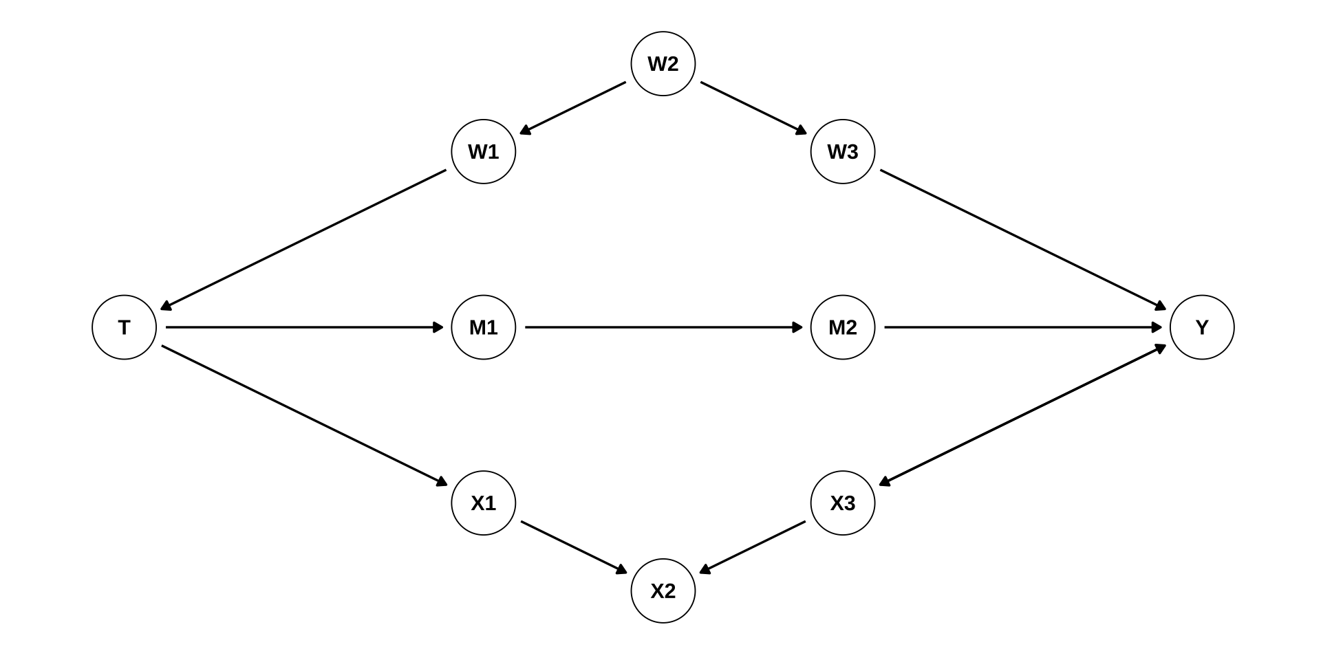
- \(T\) and \(Y\)
d-separatedconditional on- \(\emptyset\) ? 2. \(\{W_2\}\) ? 3. \(\{W_2, M_1\}\) ?
- \(\{W_1, M_2\}\) ? 5. \(\{W_1, M_2, X_2 \}\) ? 6. \(\{W_1, M_2, X_2, X_3 \}\) ?
- 1:
[1] FALSE- 2:
[1] FALSE- 3:
[1] TRUE- 4:
[1] TRUE- 5:
[1] FALSE- 6:
[1] TRUEFlow of Association and Causation - Summary
- Total association between two variables flows along all unblocked paths in a causal graph.
- Association that flows along directed, unblocked paths is causal association.
- The remaining association is non-causal association, e.g.
selection biasorconfounding association. - Causal association is asymmetric, non-causal association is symmetric.
- Causal association is a subcategory of total association.
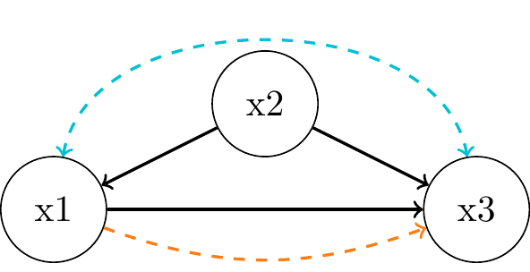
- d-separation can imply “Association is Causation`
- Ignoring the causal paths, are X and Y d-separated otherwise?
do-Operator
Structural Causal Models
- A DAG represents an underlying structural causal model:
- \(f_i\)’s can be arbitrary, non-parametric functions
- as opposed to structural equation models (SEM) in econometrics
- \(\epsilon_i\)’s are unobserved error terms
- Markovian model: all errors are assumed to be jointly independent and hence not shown in the graph.
- semi-Markovian model: some errors are correlated and shown in the graph; e.g. \(u\) in the example.
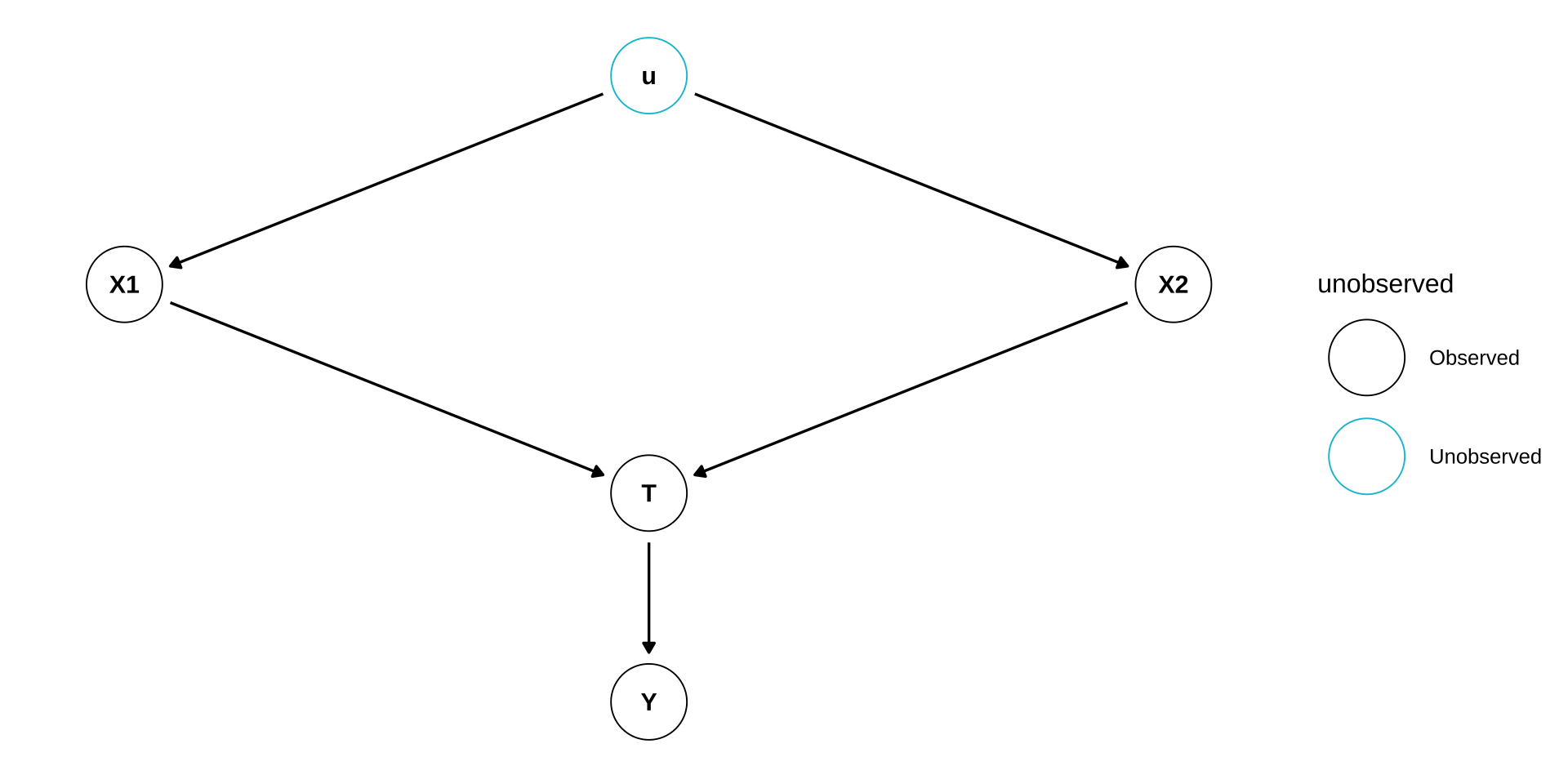
- \(Y = f_1(T, \epsilon_1)\)
- \(T = f_2(X_1, X_2, \epsilon_2)\)
- \(X_1 = f_3(u, \epsilon_3)\)
- \(X_2 = f_4(u, \epsilon_4)\)
Conditioning vs Intervention

Neal, Brady (2020). Introduction to causal inference from a Machine Learning Perspective. Course Lecture Notes (draft).
Interventions and the do-Operator
- Interventions in causal models are defined by the
do-operator. - Notation: \(P(Y|do(T = t))\) stands for:
- “probability distribution of \(Y\) if we fix \(T\) to the specific value \(t\)”.
- Interventional distributions are not the same as conditional or observational distributions.
- We can also write the
ATEwith it: \[\text{ATE} = \mathbb{E}[Y(1)] - \mathbb{E}[Y(0)] = \mathbb{E}[Y|do(T = 1)] - \mathbb{E}[Y|do(T = 0)]\] - Many (if not most) questions we try to answer with data involve some form of intervention, treatment, or action:
- P(Performance | do(Training))
- P(Sales | do(Incentive))
- P(Click-through Rate | do(Advertising))
- P(Churn | do(Call Center))
Interventions and the do-Operator
- In graphical models, intervening on a variable X is similar to a kind of surgery in which we remove all edges into that variable:
- Pre-Intervention
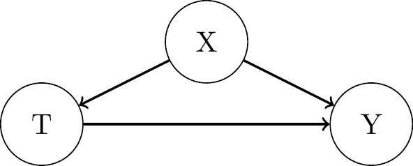
- \(Y = f_y(T, X, \epsilon_y)\)
- \(T = f_2(X, \epsilon_T)\)
- \(X = f_3(\epsilon_X)\)
- Post-Intervention
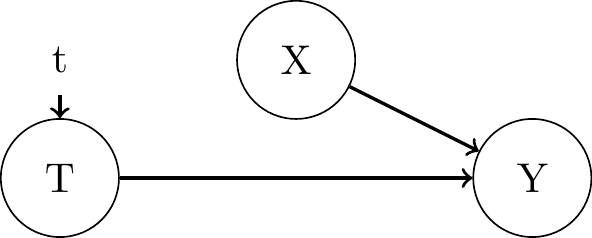
- \(Y = f_y(T, X, \epsilon_y)\)
- \(T = t\)
- \(X = f_3(\epsilon_X)\)
Interventions and the do-Operator
- Bayesian network factorization of the pre-intervention DAG:
- \(P(Y, T, X) = P(X)P(T|X)P(Y|T,X)\)
- If we intervene on \(T\) and set it to \(t\), the factorization changes:
- \(P(Y, X | do(T = t)) = P(X)P(Y|T = t, X)\)
- Marginalizing out \(X\) gives the interventional distribution of \(Y\):
- \(P(Y | do(T = t)) = \sum_{x} P(Y|T = t, X = x)P(X = x)\)
- To obtain the causal effect, we condition on the values of \(X\) and average over the distribution.
- We only obtain the associational counterpart \(P(Y|T = t)\) if \(P(X)\) would have to be replaced by \(P(X|T = t)\).
- Then: \(\sum_{x} P(Y|T = t, X = x)P(X|T = t) = \sum_{x} P(Y, X|T = t) = P(Y| T= t)\)
Interventions and the do-Operator
- Carrying out an intervention ourselves, in a randomized control trial, is not always feasible (too expensive, impractical, or unethical).
- How can we then identify the effect of interventions purely from observational data?
- We want to know \(P(Y|do(T = t))\) but all we have is data \(P(Y,X,T)\).
- And we know that \(P(Y|do(T = t) \neq P(Y|T))\) (i.e. “correlation is not causation”).
- No fancy machine learning algorithm will ever (?) solve this problem.
- One way is to find a way to transform \(P(Y|do(T = t))\) into an expression that only contains observed, “do-free” quantities.
Backdoor Adjustment
Backdoor Adjustment
- The backdoor criterion is a graphical condition that allows us to identify causal effects from observational data.
Definition 2.5: “Backdoor Criterion”
A set of variables \(W\) satisfies the backdoor criterion relative to \(T\) and \(Y\) if the following are true:
\(W\) blocks all backdoor paths between \(T\) and \(Y\) that contains an arrow into \(T\).
\(W\) does not contain any descendants of \(T\).
- If a set of variables \(W\) satisfies the backdoor criterion for \(T\) and \(Y\), then the causal effect is given by: \(P(Y|\text{do}(T = t)) = \sum_{W} P(Y|T = t, W = w)P(W = w)\).
- i.e. condition on the values of \(W\) and average over their joint distribution
Backdoor Adjustment: Proof
- Conditioning on the variables \(W\) and marginalizing them out:
- \(P(Y|\text{do}(T = t)) = \sum_{W} P(Y|\text{do}(T = t), W = w)P(W| \text{do}(T = t))\)
- Get rid of the first “do” by using the definition of the do-operator - “all backdoor paths blocked”:
- \(\sum_{W} P(Y|\text{do}(T = t), W = w)P(W| \text{do}(T = t)) = \sum_{W} P(Y|T = t, W = w)P(W| \text{do}(T = t))\)
- Get rid of the second “do” by using the definition of the do-operator - “no descendants of T in W”:
- \(\sum_{W} P(Y|T = t, W = w)P(W| \text{do}(T = t)) = \sum_{W} P(Y|T = t, W = w)P(W)\)
Backdoor Adjustment: Example
Show code
library(ggdag)
library(ggplot2)
dag <- dagify(
  T ~ X1 + X2,
  X6 ~ T,
  X2 ~ X3,
  X1 ~ X3 + X4,
  X5 ~ X4,
  Y ~ X1 + X5 + X6,
  exposure = "T", outcome = "Y",
  coords = list(
    x = c(T = 0, X1 = 1, X2 = 0, X3 = 0, X4 = 2, X5 = 2, X6 = 1, Y = 2),
    y = c(T = 0, X1 = 1, X2 = 1, X3 = 2, X4 = 2, X5 = 1, X6 = 0, Y = 0)
  )
)

dag %>%
  ggplot(aes(x = x, y = y,
             xend = xend, yend = yend)) +
  geom_dag_text(color = "black") +
  geom_dag_edges() +
  geom_dag_point(shape = 1) +
  theme_dag()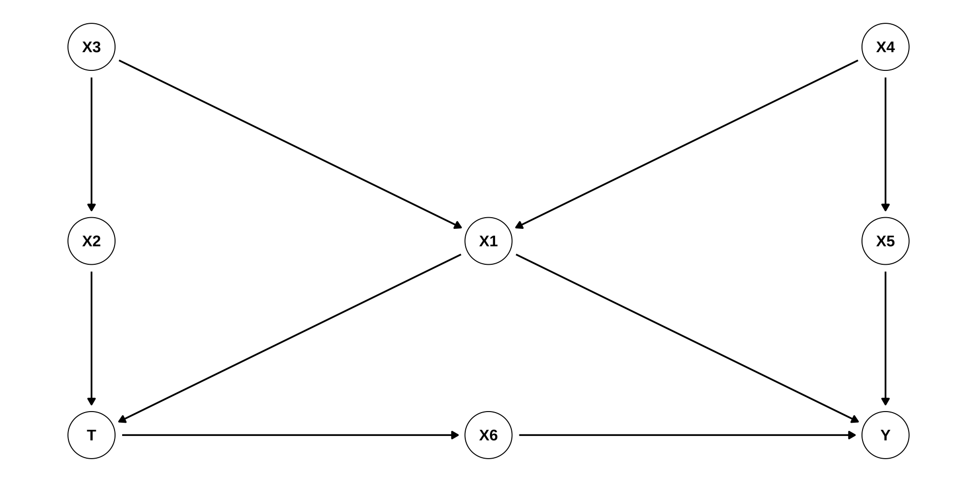
- Minimum sufficient adjustment sets?
Show code
library(ggdag)
library(ggplot2)
dag <- dagify(
  T ~ X1 + X2,
  X6 ~ T,
  X2 ~ X3,
  X1 ~ X3 + X4,
  X5 ~ X4,
  Y ~ X1 + X5 + X6,
  exposure = "T", outcome = "Y",
  coords = list(
    x = c(T = 0, X1 = 1, X2 = 0, X3 = 0, X4 = 2, X5 = 2, X6 = 1, Y = 2),
    y = c(T = 0, X1 = 1, X2 = 1, X3 = 2, X4 = 2, X5 = 1, X6 = 0, Y = 0)
  )
)

adjustmentSets(dag)
{ X1, X5 }
{ X1, X4 }
{ X1, X3 }
{ X1, X2 }Relation to the Potential Outcomes Framework
- ATE in the PO framework:
- \(\tau = \mathbb{E}[Y_i(1)] - \mathbb{E}[Y_i(0)] = \mathbb{E_X}[\mathbb{E}[Y_i|T_i=1, X_i] - \mathbb{E}[Y_i|T_i=0, X_i]]\)
- do-notation \(\mathbb{E}(Y|do(T = t))\) just another notation for the potential outcomes \(\mathbb{E}[Y(t)]\).
- Expectations and discrete treatement vs. probability weighted averages and continuous/ multi-valued treatments.
- The backdoor criterion is a graphical condition to identify valid adjustment sets for the potential outcomes framework.
- But we had no way of knowing how to choose \(W\) such that it gives us conditional exchangeability.
- The backdoor criterion is a graphical condition to choose a valid \(W\).
- It is neither necessary nor suffcient to condition on all variables in the data and model.
- Can even be harmful to condition on a (collider) variable.
- Once we have found an admissible adjustment set, we can estimate the causal effect by matching, inverse probability weighting, or linear regression (if you’re willing to assume linearity).
| Thank you for your attention! | |
 
|
|
Causal Data Science: (2) Graphical Causal Models